

EXPAND ALL
- Home
- About Pixie
- Installing Pixie
- Using Pixie
- Tutorials
- Reference

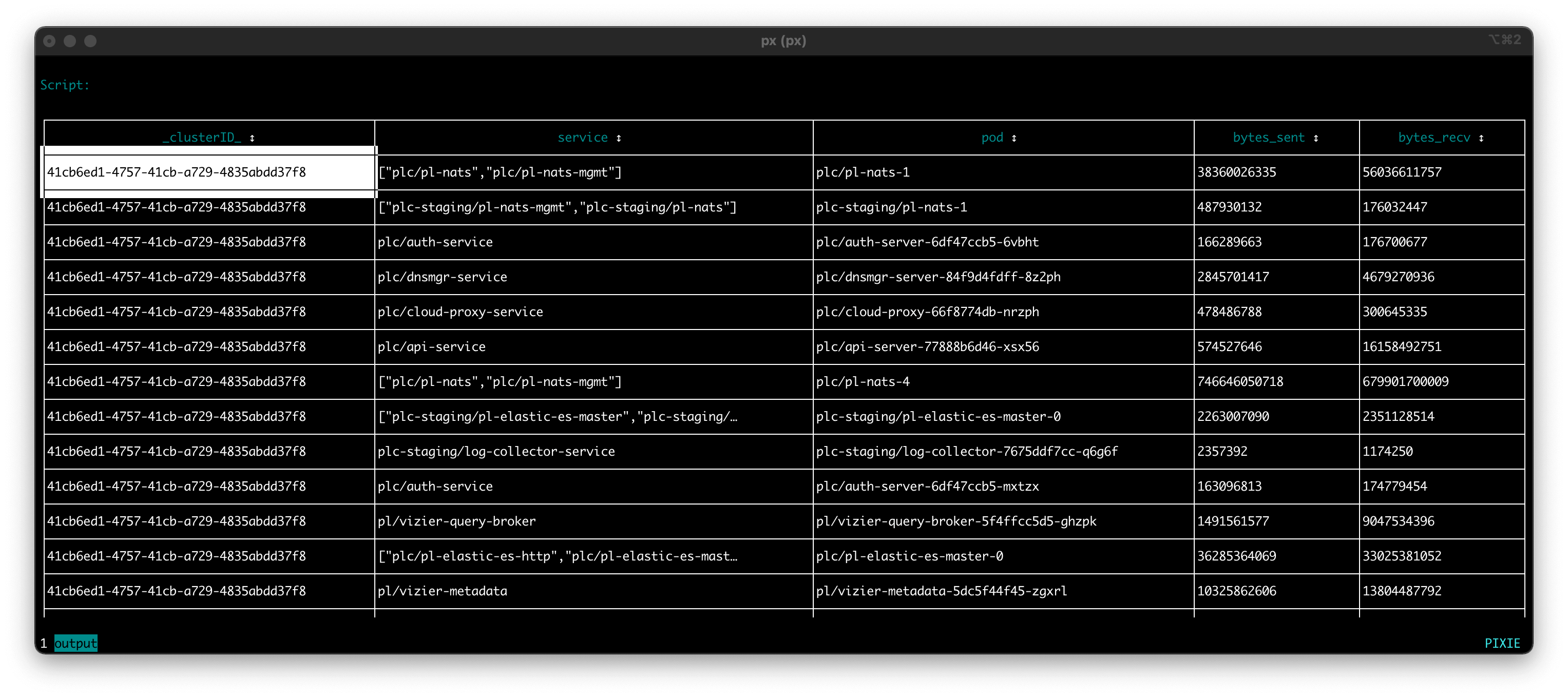
In Tutorial #1 and Tutorial #2 we wrote a simple PxL script that produced a table summarizing the total traffic coming in and out of each of the pods in your cluster. We used the Pixie CLI tool to execute the script:
In this tutorial series, we will look at other ways to visualize this data, including a time series chart and graph. We will use the Live UI to execute the script since it offers rich visualizations that are not available with Pixie's CLI or API.
The Live UI's Scratch Pad is designed for developing quick, one-off scripts. Let's use the Scratch Pad to run the PxL script we developed in Tutorial #2.
Open Pixie's Live UI.
Select the Scratch Pad script from the script drop-down menu in the top left.
Open the script editor using the keyboard shortcut: ctrl+e (Windows, Linux) or cmd+e (Mac).
Replace the contents of the PxL Script tab with the script developed in Tutorial #2:
1# Import Pixie's module for querying data2import px34# Load the last 30 seconds of Pixie's `conn_stats` table into a Dataframe.5df = px.DataFrame(table='conn_stats', start_time='-30s')67# Each record contains contextual information that can be accessed by the reading ctx.8df.pod = df.ctx['pod']9df.service = df.ctx['service']1011# Calculate connection stats for each process for each unique pod.12df = df.groupby(['service', 'pod', 'upid']).agg(13 # The fields below are counters per UPID, so we take14 # the min (starting value) and the max (ending value) to subtract them.15 bytes_sent_min=('bytes_sent', px.min),16 bytes_sent_max=('bytes_sent', px.max),17 bytes_recv_min=('bytes_recv', px.min),18 bytes_recv_max=('bytes_recv', px.max),19)2021# Calculate connection stats over the time window.22df.bytes_sent = df.bytes_sent_max - df.bytes_sent_min23df.bytes_recv = df.bytes_recv_max - df.bytes_recv_min2425# Calculate connection stats for each unique pod. Since there26# may be multiple processes per pod we perform an additional aggregation to27# consolidate those into one entry.28df = df.groupby(['service', 'pod']).agg(29 bytes_sent=('bytes_sent', px.sum),30 bytes_recv=('bytes_recv', px.sum),31)3233# Filter out connections that don't have their service identified.34df = df[df.service != '']3536# Display the DataFrame with table formatting37px.display(df)
Run the script using the keyboard shortcut: ctrl+enter (Windows, Linux) or cmd+enter (Mac).
Hide the script editor using the keyboard shortcut: ctrl+e (Windows, Linux) or cmd+e (Mac).
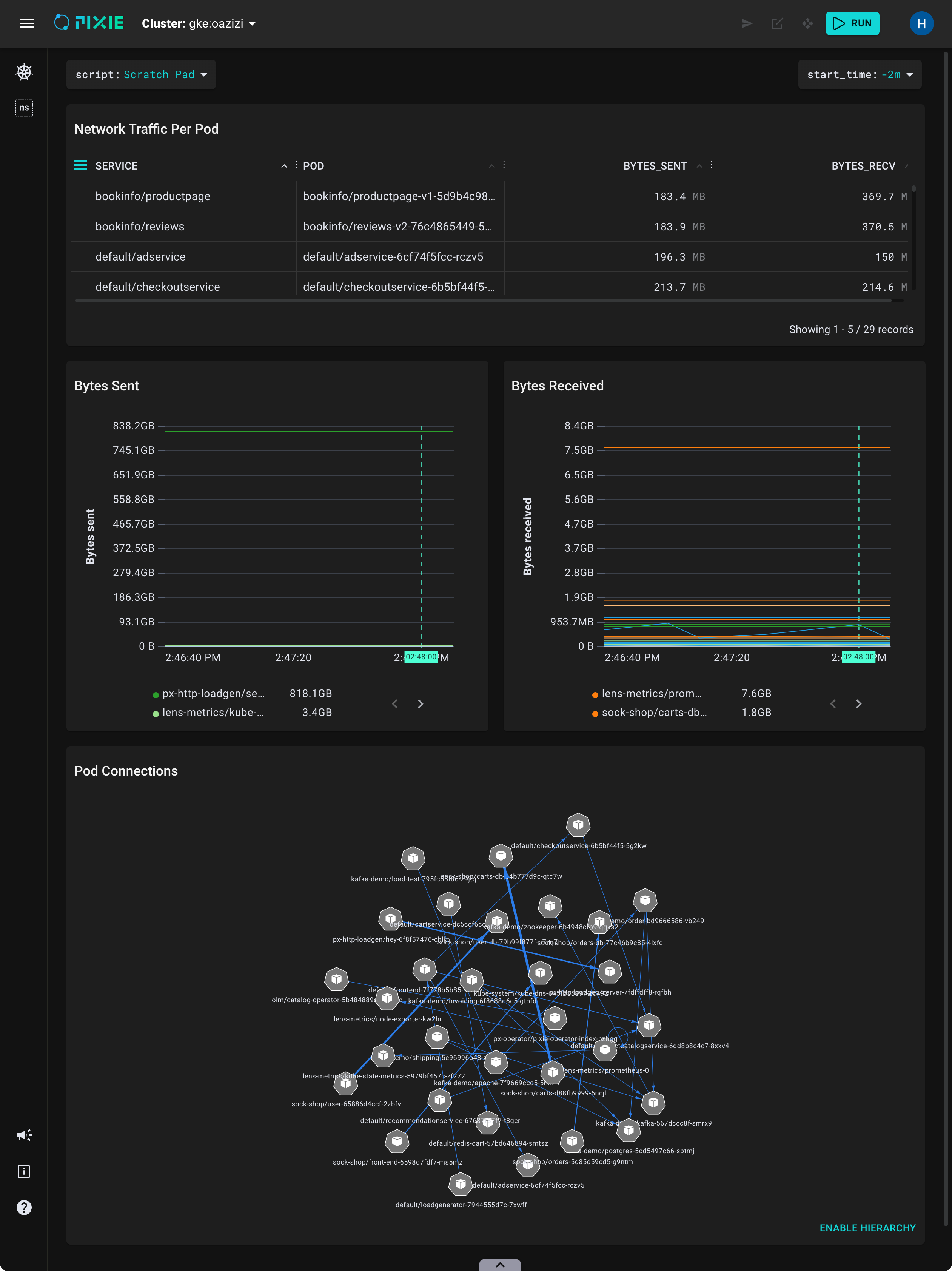
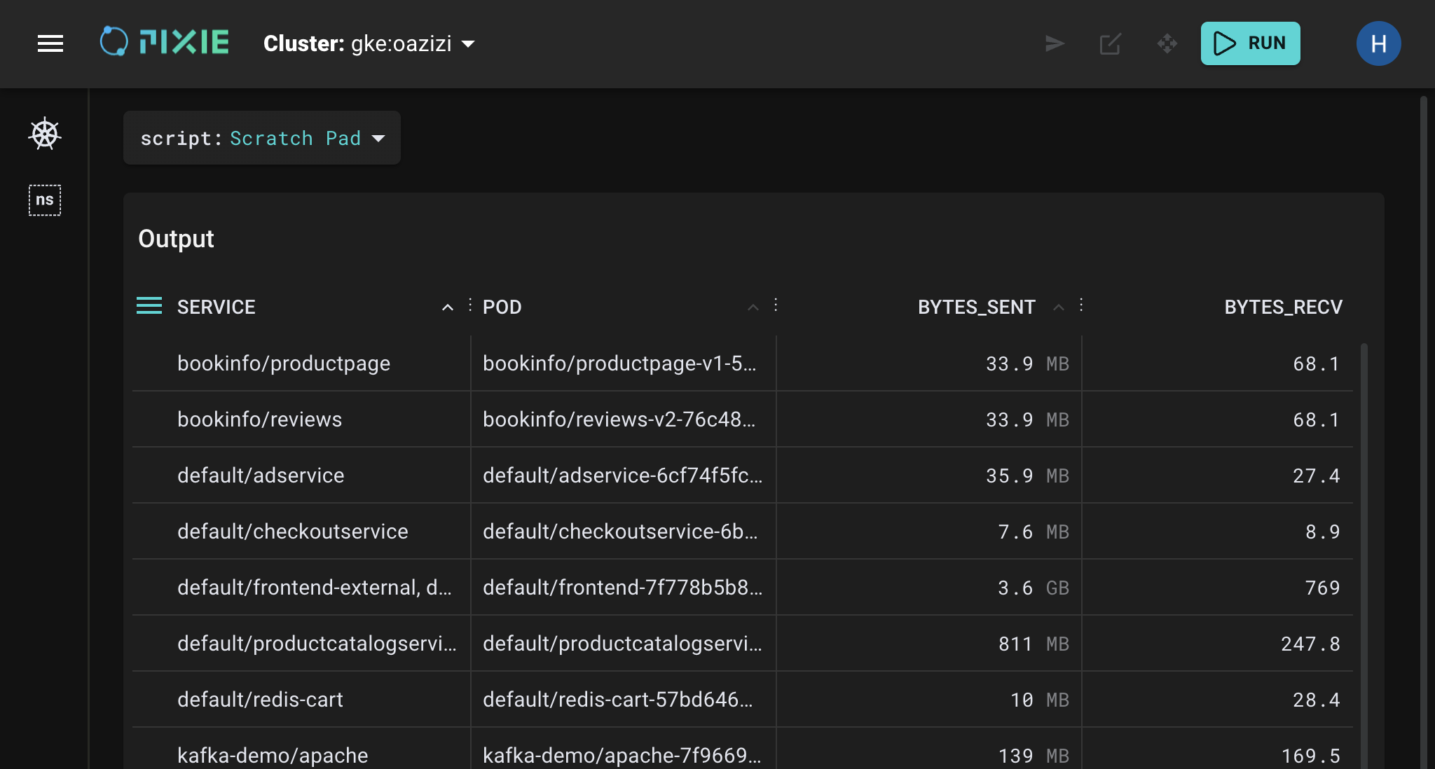
Your Live UI should output something similar to the following:
Now you know how to run PxL scripts using both the CLI and the Live UI scratch pad.
Pixie's Live UI constructs "Live View" dashboards using two files:
PxL Script queries the Pixie platform for telemetry data.Vis Spec defines the functions to execute from the PxL script, provides inputs to those functions, and defines how to visualize the output.You might wonder how our PxL Script (which does not yet have a Vis Spec) was able to be visualized in the Live UI. The Live UI allows you to omit the Vis Spec if you call px.display() in your PxL Script. This call tells the Live UI to format the query output into a table.
The last line of our PxL script includes a call to px.display(). Let's remove this function call and instead use a Vis Spec to do the same thing: format the query output into a table.
Remember that the Vis Spec specifies which function(s) to execute from the PxL script. So we will need to refactor our PxL script to contain a function with our query.
Open the script editor using the keyboard shortcut: ctrl+e (Windows, Linux) or cmd+e (Mac).
Replace the contents of the PxL Script tab with the following:
1# Import Pixie's module for querying data2import px34def network_traffic_per_pod(start_time: str):56 # Load the `conn_stats` table into a Dataframe.7 df = px.DataFrame(table='conn_stats', start_time=start_time)89 # Each record contains contextual information that can be accessed by the reading ctx.10 df.pod = df.ctx['pod']11 df.service = df.ctx['service']1213 # Calculate connection stats for each process for each unique pod.14 df = df.groupby(['service', 'pod', 'upid']).agg(15 # The fields below are counters per UPID, so we take16 # the min (starting value) and the max (ending value) to subtract them.17 bytes_sent_min=('bytes_sent', px.min),18 bytes_sent_max=('bytes_sent', px.max),19 bytes_recv_min=('bytes_recv', px.min),20 bytes_recv_max=('bytes_recv', px.max),21 )2223 # Calculate connection stats over the time window.24 df.bytes_sent = df.bytes_sent_max - df.bytes_sent_min25 df.bytes_recv = df.bytes_recv_max - df.bytes_recv_min2627 # Calculate connection stats for each unique pod. Since there28 # may be multiple processes per pod we perform an additional aggregation to29 # consolidate those into one entry.30 df = df.groupby(['service', 'pod']).agg(31 bytes_sent=('bytes_sent', px.sum),32 bytes_recv=('bytes_recv', px.sum),33 )3435 # Filter out connections that don't have their service identified.36 df = df[df.service != '']3738 return df
On
line 4we define a function callednetwork_traffic_per_pod(). This function takes a string input variable calledstart_timeand encapsulates the same query logic from the previous version of our PxL script.
On
line 7we pass the function'sstart_timeargument to the DataFrame's ownstart_timevariable.
Now, let's write the Vis Spec.
Vis Spec tab at the top of the script editor.You should see the following empty Vis Spec:
1{2 "variables": [],3 "widgets": [],4 "globalFuncs": []5}
A Vis Spec is a json file containing three lists:
- widgets: the visual elements to show in the Live View (e.g. chart, map, table)
- globalFuncs: the PxL script functions that output data to be displayed by the widgets
- variables: the input variables that can be provided to the PxL script functions
Vis Spec tab with the following:1{2 "variables": [3 {4 "name": "start_time",5 "type": "PX_STRING",6 "description": "The relative start time of the window. Current time is assumed to be now",7 "defaultValue": "-5m"8 }9 ],10 "widgets": [11 {12 "name": "Network Traffic per Pod",13 "position": {14 "x": 0,15 "y": 0,16 "w": 12,17 "h": 318 },19 "func": {20 "name": "network_traffic_per_pod",21 "args": [22 {23 "name": "start_time",24 "variable": "start_time"25 }26 ]27 },28 "displaySpec": {29 "@type": "types.px.dev/px.vispb.Table"30 }31 }32 ],33 "globalFuncs": []34}
Remember that the Vis Spec has three purposes. It defines the functions to execute from the PxL script, provides inputs to those functions, and describes how to visualize the query output.
Starting on
line 2we list a single variable calledstart_time. This input variable is provided to thenetwork_traffic_per_pod()function online 24. The Live UI will display all script variables at the top of the Live View.
Starting on
line 10we list a single table widget:
- The
namefield is an optional string that is displayed at the top of the widget in the Live View. A widget'snamemust be unique across all widgets in a given Vis Spec.- The
positionfield specifies the location and size of the widget within the Live View.- The
funcfield provides the name of the PxL script function to invoke to provide the output to be displayed in the widget. This function takes the previously definedstart_timevariable as an input argument.- The
displaySpecfield specifies the widget type (Table, Bar Chart, Graph, etc)
This Vis Spec only contains a single function, so we define it inline within the widget (starting on
line 19). If multiple widgets used the same function, you would want to define it in the"globalFuncs"field. You'll see how to do that in Tutorial #4.
Run the script using the keyboard shortcut: ctrl+enter (Windows, Linux) or cmd+enter (Mac).
Hide the script editor using the keyboard shortcut: ctrl+e (Windows, Linux) or cmd+e (Mac).
Your Live UI should output something similar to the following:
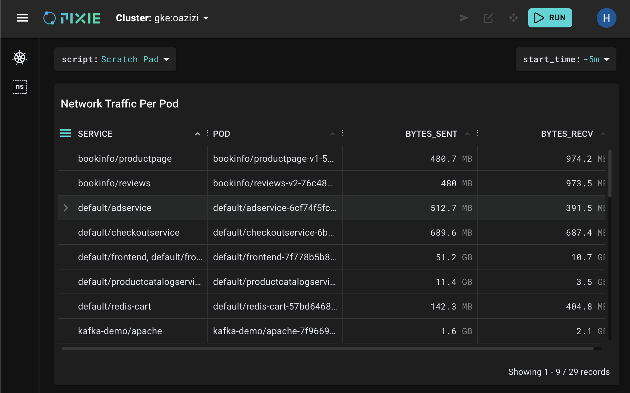
start_time variable in the top right. Select the drop-down arrow next to it, type -1h and press Enter. The Live UI should update the results to reflect the new time window.Let's add another variable, a required one, to the Vis Spec. A required variable must be input before the script can be run.
Open the script editor using the keyboard shortcut: ctrl+e (Windows, Linux) or cmd+e (Mac).
Select the PxL Script tab and replace the contents with the following:
1# Import Pixie's module for querying data2import px34def network_traffic_per_pod(start_time: str, ns: px.Namespace):56 # Load the `conn_stats` table into a Dataframe.7 df = px.DataFrame(table='conn_stats', start_time=start_time)89 # Each record contains contextual information that can be accessed by the reading ctx.10 df.pod = df.ctx['pod']11 df.service = df.ctx['service']12 df.namespace = df.ctx['namespace']1314 # Filter connections to only those within the provided namespace.15 df = df[df.namespace == ns]1617 # Calculate connection stats for each process for each unique pod.18 df = df.groupby(['service', 'pod', 'upid']).agg(19 # The fields below are counters per UPID, so we take20 # the min (starting value) and the max (ending value) to subtract them.21 bytes_sent_min=('bytes_sent', px.min),22 bytes_sent_max=('bytes_sent', px.max),23 bytes_recv_min=('bytes_recv', px.min),24 bytes_recv_max=('bytes_recv', px.max),25 )2627 # Calculate connection stats over the time window.28 df.bytes_sent = df.bytes_sent_max - df.bytes_sent_min29 df.bytes_recv = df.bytes_recv_max - df.bytes_recv_min3031 # Calculate connection stats for each unique pod. Since there32 # may be multiple processes per pod we perform an additional aggregation to33 # consolidate those into one entry.34 df = df.groupby(['service', 'pod']).agg(35 bytes_sent=('bytes_sent', px.sum),36 bytes_recv=('bytes_recv', px.sum),37 )3839 # Filter out connections that don't have their service identified.40 df = df[df.service != '']4142 return df
On
line 4we add an additionalnsargument of typepx.Namespaceto our function definition.
On
line 15we use thensvariable to filter the pod connections to only those involving pods in the specified namespace.
Vis Spec tab and replace the contents with the following:1{2 "variables": [3 {4 "name": "start_time",5 "type": "PX_STRING",6 "description": "The relative start time of the window. Current time is assumed to be now",7 "defaultValue": "-5m"8 },9 {10 "name": "namespace",11 "type": "PX_NAMESPACE",12 "description": "The name of the namespace."13 }14 ],15 "widgets": [16 {17 "name": "Network Traffic per Pod",18 "position": {19 "x": 0,20 "y": 0,21 "w": 12,22 "h": 323 },24 "func": {25 "name": "network_traffic_per_pod",26 "args": [27 {28 "name": "start_time",29 "variable": "start_time"30 },31 {32 "name": "ns",33 "variable": "namespace"34 }35 ]36 },37 "displaySpec": {38 "@type": "types.px.dev/px.vispb.Table"39 }40 }41 ],42 "globalFuncs": []43}
We've updated the Vis Spec in the following ways:
- Starting on
line 9we added anamespaceargument to the list of"variables".- By omitting a
defaultValue, thenamespacevariable is designated as required; This means that the Live UI will error until you provide a value for thenamespacevariable.- On
line 11we define thenamespaceargument type asPX_NAMESPACE. By using one of Pixie's semantic types, the Live UI will suggest the cluster's available namespaces when entering a value for the variable.- Starting on
line 31, we updated thenetwork_traffic_per_pod()function to take the new variable as an argument.
Run the script using the keyboard shortcut: ctrl+enter (Windows, Linux) or cmd+enter (Mac).
Hide the script editor using ctrl+e (Windows, Linux) or cmd+e (Mac).
You should get the following error since the
Vis Specdefines thenamespaceargument as a required variable:
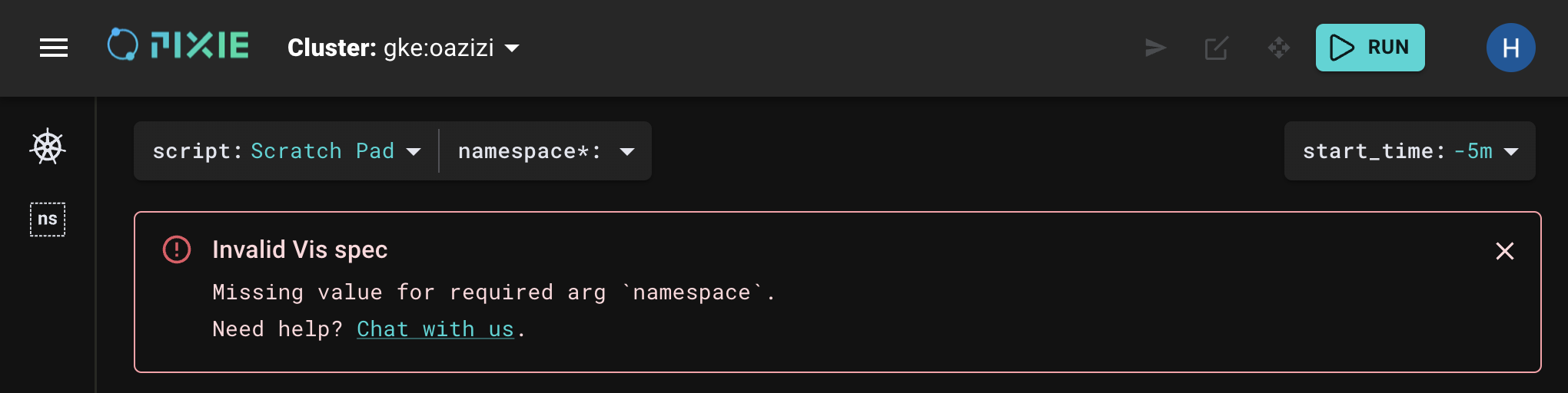
namespace argument. If you wait for a second, the drop-down menu should populate with the available namespace names. Type default and press Enter.The Live UI should update with the appropriate results for that namespace.
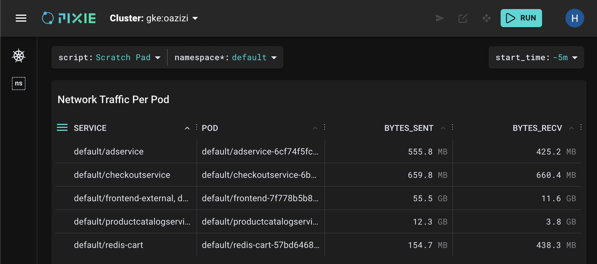
Pixie's Live View widgets are interactive. Here are a sample of ways you can interact with the table widget:
To sort a table column, click on a column title.
Click on deep links to easily navigate between Kubernetes entities. Click on any node / service / pod name (in a table cell) to be taken to an overview of that resource.
To see a table row's contents in JSON form, click on the row to expand it. This is useful for seeing the contents of a truncated table cell.
To add / remove columns from the table (without modifying the PxL script), use the hamburger menu to the left of the first column title.
Congratulations, you wrote your first Vis Spec to accompany your PxL Script!
Tables aren't all that exciting, but now that you know how Vis Specs work you can learn how to visualize your data in more interesting ways. In Tutorial #4 we'll add a timeseries chart to our Live View.
